
Quick Summary: A demonstration of computer vision techniques to create feature vectors to feed an XGBoost machine learning process which results in over 90% accuracy in recognition of the presence of a particular invasive species of plant in a photograph.
Introduction
This is an example of how to combine computer vision techniques with supervised machine learning to create a system that can recognize a class of objects. The data source is the Kaggle competition Invasive Species Monitoring, which provides 2,296 color photographs of plants in a natural habitat. The challenge is to find an automated means of classifying whether the photograph contains hydrangea plants. While these plants are sold as ornamentals, in some parts of the US they thrive as an invasive species, and their progress and growth needs to be monitored.
Much of the focus on classifying photographs in machine learning today uses deep learning techniques, a class of computationally intensive techniques, usually requiring specialized hardware which are showing some really amazing results. However, having just completed a Georgia Tech’s Computer Vision class as part of my Master’s program, I wanted to see how these techniques would fare in practice.
What you’ll see in this post is the transformation of the input photographs into a more traditional, and far more compact feature matrix. Then, these features are used in an XGBoost classification process to create an effective model that can recognize the presence of a hydrangea plant in new photos. All tools used are open source, python-based frameworks, and my scripts are available at my Github.
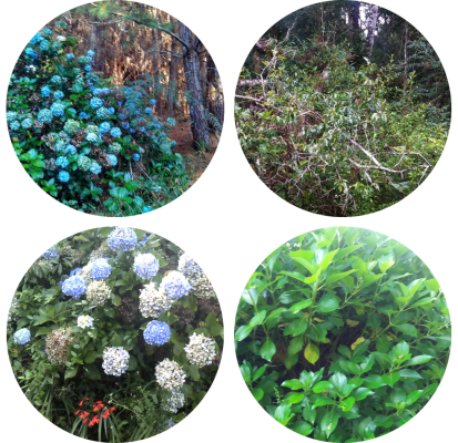
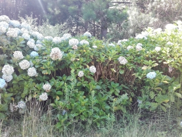
Here’s an example of one of the positive input photographs:
Feature Engineering
Due to the long runtime for feature engineering, the creation of features is separated from the running of the models. Feature engineering scripts are here.
Four main classes of features are created.
- Color histogram distance
- Custom-coded blue detector
- Template matching intensity squared differences
After reviewing some of the training images of both positive and negative classes, it was apparent that in many of the positive cases, the hydrangea plants could be recognized by their large flowering structures. These flowers tended towards blue at their peak, but could vary in color if the plant in question was pre- or post-flowering, or simply if the brightness of the image “washed-out” most of the color. So I set out to build features that would indicate the presence of the unique shape and color of the flowering bodies.
First, I needed to find positive examples within the images that would highlight the presence of the invasive hydrangea. I selected 8 training images, and manually cut out patches that represented a good feature (18 training patches total). Clearly, there is a lot of subjectivity in this step, and I am by no means an expert in these flowers, but I needed to start somewhere.
Here’s a couple examples of the patches used as training images for the next steps:


Structure of images
I used OpenCV for most of the image handing. Within OpenCV, the typical representation of an image is a 3-layer Numpy array. Each layer represents the intensity of blue, green and red values at each pixel location. When viewing the image, we only observe a single pixel, but the rendering is built using these three values. Therefore, we can directly used these color values as a source of information.
Color Histogram Distances
For each of the training patches, I created a histogram of the patch’s BGR (blue, green, red) values. I then broke each whole image into 60×60 segments and calculated the histogram for that patch. After excluding low values (I didn’t want to match on dark segments of the photo), and normalizing these histograms to a consistent range, I calculated and recoded the Euclidian distances between then. Therefore, if one of the 60×60 input segments has a very similar distribution of color values to one of the input templates, the Euclidean distance would be low, and vise versa. The histogram approach is robust to small differences in scale, orientation or rotation. As the goal of this analysis is to detect the presence of hydrangea, without needing to localize it within the image, the features created are both the minimum distance between a template and the image, and the number of 60×60 segments below various threshold levels.
OpenCV supports multiple color spaces, which are different ways of encoding color and intensity other than the traditional BGR layers. I also converted the templates and the images into the HSV color space, and built a series of histogram distance features using the H (hue) and S (saturation) channels, to see if this approach might be more robust to the variation in lighting.
Custom-Coded Blue Detector
To develop a bit of an intuitive feel for the raw photographic data, I opened up several images in GIMP, which allows to easily navigate parts of the image to explore the underlying values. It was apparent that the relationships between the BGR values on a full-bloomed and properly exposed image of a hydrangea flower were unique – very high blue values and mid-to-low green and red. So I built a quick function in Numpy, working directly with the photo’s matrix values that counted the number of pixels in each segment where there were very high blue values with low green and red, and recorded the highest proportion found in each image.
Template Matching Intensity
OpenCV has a powerful function, cv2.matchTemplate(), which will take a smaller image, and slide it across a larger image, calculating the differences for each position. This approach has it yield the normalized squared differences between the two vectors, but there are several metrics to choose from. Here, the program uses the smoothed greyscale versions of the patches to speed computation, and as the first two metrics are already analyzing the color content well. This function is very fast, but the approach suffers if the scale or orientation of the being tracked is too different.
Features Created
This approach produced a series of features for each input template, plus one overall measure for the blue detector, resulting in 165 independent features for use in machine learning. This process takes a long time to run (several hours on my MacBook), but once it’s completed, we have a very compact set of features (less than 3.5 Mb) that represents 2.3 Gb worth of jpegs.
Machine Learning Approach
Code for the ML steps are here, and assume that features have already been run and saved as above.
For this project, I’ll use XGBoost (Extreme Gradient Boosting), the library that has been at the top of so many Kaggle competitions since it came out. It’s fast and powerful, but very sensitive to the parameter settings. Initially I used CVGrid and RandomForestClassifier (RFC), just to make sure I was on the right track with the features. RFC is very nice in that it generally produces good results with minimal tuning, so it provided a quick check that things were working the way I wanted them to.
Once I moved to XGBoost, I first used its cross-validation function to tune the parameter settings. For this project, I chose AUC (“area under the curve”) as the evaluation metric, rather than a simpler accuracy rate. AUC is sensitive to the strength of the recommendation, and better accounts for the fact that some classifications could be randomly right in any sample. It’s both more stringent than accuracy rate, and more finely calibrated.
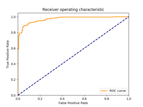
Once I arrived at my parameter settings, tuning the number of booster iterations, level of regularization, learning rate and random sampling, I split the data 80/20 into train and test segments. This would be expected to have similar AUC measurements as the cv-experiments, but will let us calculate a final accuracy rate and create a ROC chart.
Results
The AUC matrix in cross-validation was .954, which was very encouraging. I then split the data into train/test samples and built the XGBoost model on the training set with the parameters defined in the cross-validation experiment. When I used this model to predict the probability of the presence of a hydrangea plant on the holdout testing sample, it resulted in an AUC of .971. Using these probabilities to make firm predictions resulted in an accuracy rate of 90.4%, with the breakdown below.
Correctly classified, no hydrangea:141
Correctly classified, with hydrangea:273
Incorrectly classified, no hydrangea:24
Incorrectly classified, with hydrangea:20
Next Steps
To improve the performance of this process, I would suggest two areas for next steps:
Input feature patches: Experimentation with what feature patches work best, and manual selection/cleaning of the patches should provide better accuracy. I wanted to build this as a minimum viable product to see what kind of results the algorithm could produce, so the input patches are pretty simple selections without cleaning of extraneous features, beyond a little simple Gaussian blurring.
Parallelization of feature creation: Creation of the feature vector is the long pole in this process, but clock time could be significantly improved by parallelizing the image processing. Individual images have no bearing on each other in the image processing, so there is no reason this couldn’t be parallelized, either on a single computer, or across a cluster, for a significant speedup.
